3 Modeling

3.1 Logistic Regression Modeling

Address class imbalance by up‐weighting the minority “Bad” class.
Train a weighted logistic regression model on all features.
Diagnose model fit via summary and check multicollinearity (VIF).
Compute and visualize feature importance to see which predictors drive the model.

Code

train_data <- readRDS("train_data.rds")
test_data  <- readRDS("test_data.rds")
model_weights <- ifelse(train_data$CreditRisk == "Bad",
                       sum(train_data$CreditRisk == "Good")/sum(train_data$CreditRisk == "Bad"),
                       1)
lr_model <- glm(CreditRisk ~ .,
               data = train_data,
               family = binomial,
               weights = model_weights)
summary(lr_model)
car::vif(lr_model)

library(caret)
library(tibble)
library(dplyr)
library(ggplot2)

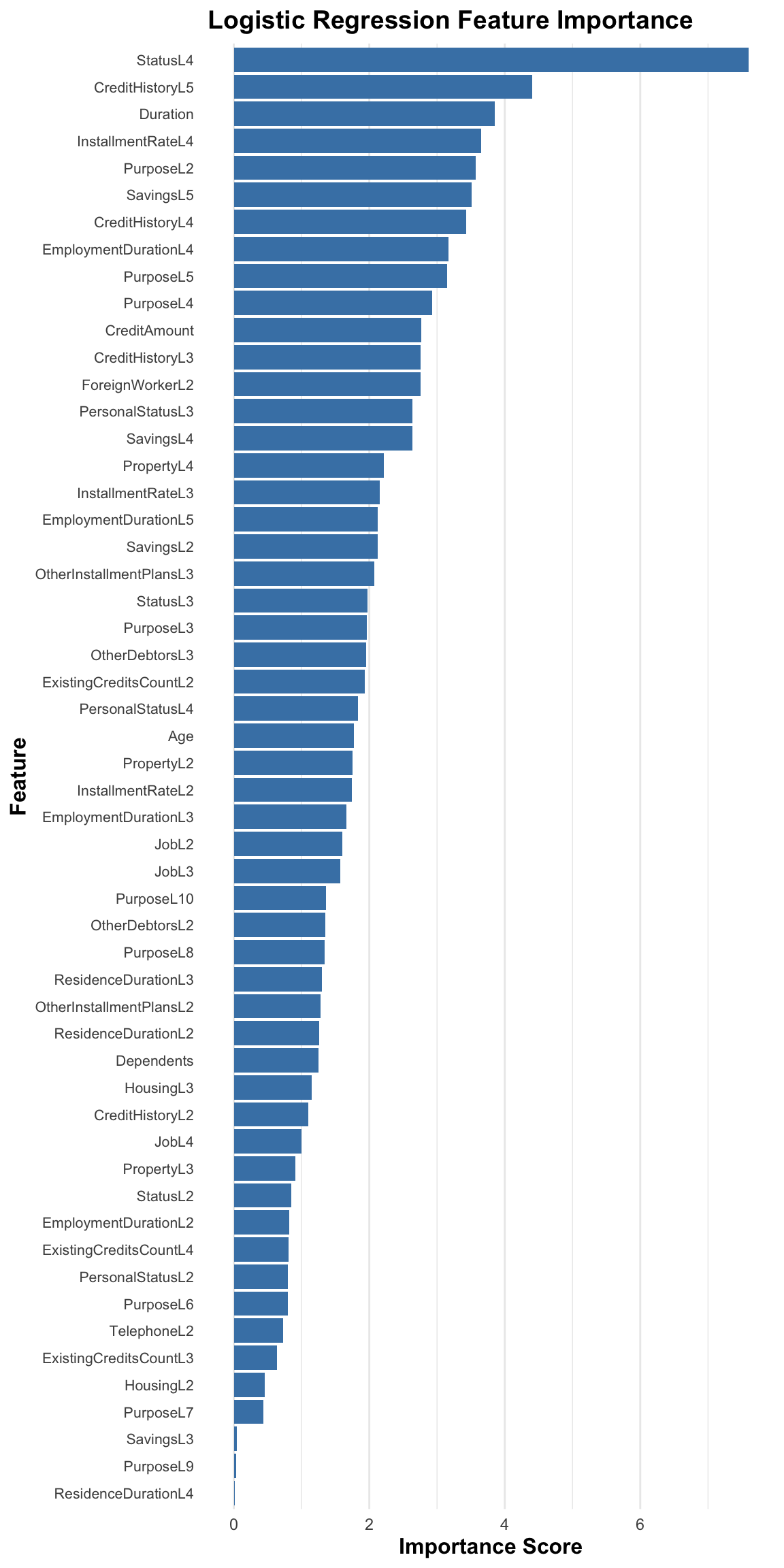
lr_importance <- varImp(lr_model)

imp_df <- lr_importance %>%
  rownames_to_column("Feature") %>%
  rename(Importance = Overall)

ggplot(imp_df, aes(x = Importance, y = reorder(Feature, Importance))) +
  geom_col(fill = "steelblue") +
  labs(
    title = "Logistic Regression Feature Importance",
    x     = "Importance Score",
    y     = "Feature"
  ) +
  theme_minimal() +
  theme(
    plot.title         = element_text(size = 14, face = "bold"),
    axis.title         = element_text(size = 12, face = "bold"),
    axis.text.y        = element_text(size = 8, margin = margin(r = 5)),
    panel.grid.major.y = element_blank()
  )

   Top feature importance from the logistic regression model

Status
CreditHistory
Duration
InstallmentRate

3.2 Decision Tree Model

Define tree complexity and cross‐validation parameters.
Train a classification tree using information‐gain splits.
Prune the tree at the CP value minimizing cross‐validated error.
Visualize the pruned tree to inspect decision rules and compare to LIME/SHAP explanations.

Code

library(rpart)
library(rpart.plot)
tree_control <- rpart.control(
  minsplit = 20,
  minbucket = round(20/3),
  cp = 0.005,
  maxdepth = 4,
  xval = 10
)

tree_model <- rpart(
  CreditRisk ~ .,
  data = train_data,
  method = "class",
  parms = list(split = "information"),
  control = tree_control
)

best_cp <- tree_model$cptable[which.min(tree_model$cptable[, "xerror"]), "CP"]
pruned_tree <- prune(tree_model, cp = best_cp)

rpart.plot(pruned_tree, 
           type = 5, 
           extra = 106,
           box.palette = "GnBu",
           shadow.col = "gray")

     classification rules for decision tree

Status
Duration
Savings
CreditHistory

3.3 Model Evaluation on Test Set

Logistic Regression: predict probabilities, classify at 0.5 threshold, and compute confusion matrix treating “Bad” as the positive class.
Decision Tree: predict class labels and compute confusion matrix similarly.

Code

library(caret)
lr_pred <- predict(lr_model, test_data, type = "response")
lr_pred_class <- factor(ifelse(lr_pred > 0.5, "Good", "Bad"),
                       levels = c("Bad", "Good"))
lr_conf <- confusionMatrix(lr_pred_class, test_data$CreditRisk, positive = "Bad")


tree_pred <- predict(pruned_tree, test_data, type = "class")
tree_conf <- confusionMatrix(tree_pred, test_data$CreditRisk, positive = "Bad")

3.3.1 Confusion Matrices

Code

# Load required packages
library(dplyr)
library(ggplot2)

# 1. Tidy up the confusion tables
tbl_lr <- as.data.frame(lr_conf$table) %>%
  rename(Actual = Reference, Predicted = Prediction, Count = Freq) %>%
  mutate(Model = "Logistic Regression")

tbl_tree <- as.data.frame(tree_conf$table) %>%
  rename(Actual = Reference, Predicted = Prediction, Count = Freq) %>%
  mutate(Model = "Decision Tree")

cm_vis_df <- bind_rows(tbl_lr, tbl_tree)

# 2. Plot side-by-side heatmaps
ggplot(cm_vis_df, aes(x = Actual, y = Predicted, fill = Count)) +
  geom_tile(color = "white") +
  geom_text(aes(label = Count), size = 5) +
  facet_wrap(~ Model) +
  scale_fill_gradient(low = "white", high = "steelblue") +
  labs(
    title = "Logistic Regression vs. Decision Tree",
    x     = "Actual Class",
    y     = "Predicted Class",
    fill  = "Count"
  ) +
  theme_minimal() +
  theme(
    plot.title    = element_text(size = 14, face = "bold"),
    axis.title    = element_text(size = 12),
    axis.text     = element_text(size = 10),
    strip.text    = element_text(size = 12, face = "bold"),
    panel.grid    = element_blank()
  )

Logistic Regression demonstrates stronger predictive performance compared to the Decision Tree.
Decision Tree struggles more with false positives, while Logistic Regression has higher accuracy and reliability in predictions.

3.3.2 ROC Analysis

Code

library(pROC)
library(ggplot2)
lr_probs <- predict(lr_model, test_data, type = "response")
roc_lr <- roc(response = test_data$CreditRisk, 
              predictor = lr_probs,
              levels = c("Bad", "Good"),
              direction = "<")
plot(roc_lr, 
     print.auc = TRUE, 
     auc.polygon = TRUE, 
     max.auc.polygon = TRUE,
     grid = TRUE,
     print.thres = "best", 
     main = "Logistic Regression ROC Curve")

Code

tree_probs <- predict(pruned_tree, test_data, type = "prob")[, "Bad"]
roc_tree <- roc(response = test_data$CreditRisk, 
                predictor = tree_probs,
                levels = c("Good", "Bad"),
                direction = "<")
plot(roc_tree, 
     print.auc = TRUE, 
     auc.polygon = TRUE, 
     max.auc.polygon = TRUE,
     grid = TRUE,
     print.thres = "best", 
     main = "Decision Tree ROC Curve")

Code

ggroc(list(Logistic = roc_lr, DecisionTree = roc_tree), legacy.axes = TRUE) +
  geom_abline(slope = 1, intercept = 0, linetype = "dashed", color = "red") +
  labs(title = "ROC Curve Comparison",
       x = "False Positive Rate (1 - Specificity)",
       y = "True Positive Rate (Sensitivity)") +
  theme_minimal() +
  scale_color_manual(values = c("#1f77b4", "#ff7f0e")) +
  annotate("text", x = 0.7, y = 0.3, label = paste("Logistic AUC =", round(roc_lr$auc, 3)), color = "#1f77b4") +
  annotate("text", x = 0.7, y = 0.2, label = paste("Tree AUC =", round(roc_tree$auc, 3)), color = "#ff7f0e")

ROC curves were generated to assess how well our logistic regression and decision tree models distinguish between “Bad” and “Good” credit risks across all possible classification thresholds. The plot spans a false positive rate from 0 to 1 on the x-axis and a true positive rate from 0 to 1 on the y-axis, with a dashed red diagonal representing random guessing. The decision tree’s ROC (orange line, AUC = 0.724) rises sharply at low false positive rates but then follows a near-straight line toward (1,1), indicating moderate discrimination. In contrast, the logistic regression ROC (blue line, AUC = 0.782) consistently stays above the tree’s curve—especially between FPRs of 0.05 and 0.40—demonstrating stronger sensitivity at comparable specificity levels. This comparison shows that while both models outperform random, the logistic regression provides more reliable separation of credit risk cases across thresholds.

3.3.3 Comparison of Model Performance Metrics

Model	AUC	Accuracy	Sensitivity	Specificity
Logistic Regression	0.782	0.723	0.733	0.719
Decision Tree	0.722	0.733	0.344	0.900

Logistic regression delivers superior overall discrimination and excels at identifying risky applicants by catching nearly twice as many bad cases as the decision tree. The decision tree, in contrast, more reliably approves good applicants but fails to detect the majority of high risk borrowers. As a result, when the priority is to minimize the chance of approving a bad credit, logistic regression is the preferred model; only when the cost of falsely rejecting a good borrower is overwhelmingly high might one consider the decision tree’s stronger approval rate for good applicants.